notes on the essence of linear algebra

The almost genius playlist from 3blue1brown.

vector

$\vec{v}\in {\mathbb{R}}^n$ has a mathematically rigorous definition, but for computer science, treat it as a column or a row of numbers. Each number represents a scalar along a dimension, ordered by your basis.

So in ${\mathbb{R}}^2$, $\left[\begin{array}{c}2\\ 3\end{array}\right]=2\hat{i}+3\hat{j}$.

the origin is fixed of course at $(0,0)$, and this holds for any coordinate system as long as we are not translating the origin.

basis

What is the direction and scale of “1 unit”, as I choose to define it? Default is just to use orthogonal $\hat{i}$, $\hat{j}$, and $\hat{k}$ in the default grid sense.

linearity

addition

$\left[\begin{array}{c}a\\ b\end{array}\right]=a\hat{i}+b\hat{j}$ means $a$ steps in the $\hat{i}$ direction and then $b$ steps in the $\hat{j}$ direction.

$\vec{c}=\vec{a}+\vec{b}\Rightarrow c_x=a_x+b_x,c_y=a_y+b_y$.

scalar

$\vec{v}\mapsto k\vec{v}$ means multiply length by $k$, in the same direction.

These two conditions make linearity. Formally, for a transformation $L$:

• $L(x+y)=L(x)+L(y)$
• $L(kx)=kL(x)$

A visual test is that an evenly spaced line of points remains evenly spaced after $L$.

note that origin will remain fixed

span

Defined in terms of $\vec{v}$ and $\vec{w}$.

$\mathrm{span}(\vec{v},\vec{w})=\{a\vec{v}+b\vec{w}\mid a,b\in \mathbb{R}\}$.

What surface do the possible ends draw?

matrices

Say I want to define a transformation $L$ on $\hat{i}$ and $\hat{j}$:

$$A=\left[\begin{array}{cc}L(\hat{i})& L(\hat{j})\end{array}\right]$$

The columns represent the new positions of $\hat{i}$ and $\hat{j}$ after the transform.

The effect can be a shear, scale, rotation, etc.

What would my original vector $\vec{v}$ look like? $A\vec{v}$ is the final position of the end.

You can think like this: if my $\hat{i}$ is now $2x$, I move double the steps. If my $\hat{j}$ is rotated, I do the same on $\vec{v}$.

What is interesting is:

$\vec{v}=\left[\begin{array}{c}a\\ b\end{array}\right]=a\hat{i}+b\hat{j}$.

After the transform, the same scalars still hold:

$A\vec{v}=aL(\hat{i})+bL(\hat{j})$.

For example, if $A=\left[\begin{array}{cc}2& 4\\ 3& 5\end{array}\right]$, then $A\vec{v}=a\left[\begin{array}{c}2\\ 3\end{array}\right]+b\left[\begin{array}{c}4\\ 5\end{array}\right]$.

And if you forget “vectors” and treat it like matrix multiplication, the effect is constructed to be the same.

linear independence

Defined for a set of vectors.

You can ask: does it add anything to the span? If the span remains the same even if I remove it, then it can be constructed by some linear combination of the remaining vectors.

That is, $\vec{v}\in \mathrm{span}(S\setminus \{\vec{v}\})$, so it is linearly dependent.

basis

Defined for a space, say ${\mathbb{R}}^2$ or ${\mathbb{R}}^n$.

It is the linearly independent set of vectors that span it.

dimension collapse

Say I use a transformation $A:{\mathbb{R}}^2\to {\mathbb{R}}^2$ where $L(\hat{j})$ is linearly dependent on $L(\hat{i})$.

A trivial one is $\hat{j}$ same as $\hat{i}$:

$$A=\left[\begin{array}{cc}1& 1\\ 0& 0\end{array}\right],A\left[\begin{array}{c}x\\ y\end{array}\right]=\left[\begin{array}{c}x+y\\ 0\end{array}\right]$$

So the second dimension is gone: for every input, $A(x,y)\in \mathrm{span}(\hat{i})$.

The span, which for a basis was a plane, is just a line after transformation. Note that this is not a basis change; we still describe scalars in terms of $\hat{i}$ and $\hat{j}$.

Think of it as one-way loss of information. I cannot uniquely go back from something on the line to what $(x,y)$ was before the transformation. Just like $x\cdot 0=0$, I have no way to know what $x$ could have been, except “anything”.

compositions

A transformation can be a scale, shear, rotation, reflection, projection, or a composition.

In general, $L_1{L}_2\ne L_2{L}_1$.

To read it, go right to left: $L_1{L}_2(\vec{v})=L_1(L_2(\vec{v}))$.

determinant

Under a transformation $L$, area in 2D, or volume in higher dimensions, scales by $|\det (L)|$.

Negative determinant implies orientation flip.

Think of a dimension collapse from some area in 2D to a line with 0 area. This is what it means to have a collapse when $\det (L)=0$.

For higher dimensions, collapse can be in multiple dimensions. Say $\hat{j}$ and $\hat{k}$ collapse to 0, so you have a line as span, or all collapse to 0, so just a point remains as span.

Now if you think of it as area or volume scaling, then clearly:

$\det (A)\det (B)=\det (AB)$.

Visually, $A$ then $B$ is the same as $AB$ in compositions.

linear system of equations

The good case has $n$ equations and $n$ variables. Say we have 2:

$A\vec{x}=\vec{b}$.

Think of $\vec{x}$ as the vector that I want to find. Then $A$ is a transformation defined by constants, and $\vec{b}$ is the resultant vector.

So a linear equation is: what transformation applied to $\vec{x}$ makes it the same as $\vec{b}$?

The inverse reverses the $A$ transform:

$\vec{x}=A^{-1}\vec{b}$.

Except, if $A$ collapses everything to a lower dimension, $\det (A)=0$, then we can never say for sure what the original was.

If $\vec{b}\in \mathrm{Col}(A)$, there are infinite solutions. If $\vec{b}\notin \mathrm{Col}(A)$, there is no solution.

rank

$\mathrm{rank}(A)=\dim (\mathrm{Col}(A))$.

If the transform collapses dimensions, rank decreases.

Say rank decreases by $\Delta$. If $\Delta =2$, then a whole plane has collapsed to a point.

column space

Of a transform $A$, the column space is:

$\mathrm{Col}(A)=\mathrm{span}\{\text{columns of }A\}$.

There must be some redundancy / linear dependence in the columns to collapse dimensions.

null space/kernel

Say dimensions do collapse. Then the set of vectors that got collapsed to 0 is the null space:

$\mathrm{Null}(A)=\{\vec{v}\mid A\vec{v}=\vec{0}\}$.

non-square matrices

It is very much possible to apply a transformation that changes dimensions:

$A:{\mathbb{R}}^n\to {\mathbb{R}}^m$.

I can define a linear transform $P$ as projection onto the x-axis:

$$P:{\mathbb{R}}^2\to \mathbb{R},P\left[\begin{array}{c}x\\ y\end{array}\right]=\left[\begin{array}{cc}1& 0\end{array}\right]\left[\begin{array}{c}x\\ y\end{array}\right]=x$$

Any higher-to-lower dimension transform cannot be reversed uniquely: $n>m\Rightarrow A:{\mathbb{R}}^n\to {\mathbb{R}}^m$ is not one-to-one.

What $A$ as a transform shows:

$$A\in {\mathbb{R}}^{m\times n}\Rightarrow \{\begin{array}{l}n=\text{dimension converting from}\\ m=\text{dimension converting to}\end{array}$$

dual

A dual vector is a linear transform to a scalar:

$f:{\mathbb{R}}^n\to \mathbb{R}$.

For a column vector in ${\mathbb{R}}^n$, the dual is a row of $n$ elements. The operation is just matrix multiplication to a $1\times 1$ scalar:

$$\left[\begin{array}{cccc}{a}_1& a_2& \cdots & a_n\end{array}\right]\left[\begin{array}{c}{x}_1\\ x_2\\ ⋮\\ x_n\end{array}\right]=\sum _{i=1}^n{a}_i{x}_i$$

The idea of a dual is that it lets you define, for say 2D, $f(x,y)=ax+by$, which can extract info from the vector as a linear map.

Take dot product with another vector $\vec{w}=(a,b)$. Then $f_{\vec{w}}(x,y)=ax+by$. The transform is tied to $\vec{w}$ here; it gives a signed scalar measurement along $\vec{w}$.

I feel the idea is pretty redundant

dot product

For $\vec{v},\vec{w}$, the dot product is:

$\vec{v}\cdot \vec{w}=\Vert \vec{v}\Vert \Vert \vec{w}\Vert \cos \theta$.

The scalar that it gives is the dot product.

Now $\vec{v}\cdot \vec{w}=\vec{w}\cdot \vec{v}$.

Why? Assume both are the same length. You can make a line bisecting the angle between them. In such a scenario, both $\vec{v}$ and $\vec{w}$ are interchangeable.

Now if $\vec{v}$ and $\vec{w}$ have different lengths, consider $\vec{v}=k{\vec{v}}^{\prime }$, such that ${\vec{v}}^{\prime }$ and $\vec{w}$ are the same length as above.

You get the same symmetry, with the extra factor $k$ put back. The idea visually explains dot product commutativity.

Now you can use the above dual idea to define dot as well.

Instead of dot of 2 vectors, define dot as a dual tied to one vector and applied to the other:

$f_{\vec{w}}(\vec{v})={\vec{w}}^{\top }\vec{v}$.

again a bit redundant idea unless we build on top

cross product

Geometrically, $\Vert \vec{v}\times \vec{w}\Vert$ is the area of the parallelogram enclosed by $\vec{v}$ and $\vec{w}$.

Though it is defined as a vector being the result.

In such a scenario you can technically say that cross product is not defined in 2 dimensions as a vector in the same space, since the result needs to be perpendicular and there is no space in 2 dimensions.

In 3D, it gives a perpendicular vector with magnitude equal to the area. Which orientation is then convention.

some intuition on the calculations

You can think of $\vec{x}\times \vec{y}$ as giving an area-oriented vector.

If you dot another vector $\vec{z}$ with it, it gives the volume of the 3 vectors $\vec{x},\vec{y},\vec{z}$:

$\vec{z}\cdot (\vec{x}\times \vec{y})=\det (\vec{z},\vec{x},\vec{y})$.

Now say I want to find that perpendicular vector and I have $\vec{x}$ and $\vec{y}$.

I can define a 3D to 1D transform as:

$f(\vec{z})=\det (\vec{z},\vec{x},\vec{y})$.

Magnitude wise, this determinant is the same as dot of $\vec{z}$ and the cross product $\vec{p}$:

$f(\vec{z})=\vec{z}\cdot \vec{p}$, where $\vec{p}=\vec{x}\times \vec{y}$.

Now if you dot and compare coefficients:

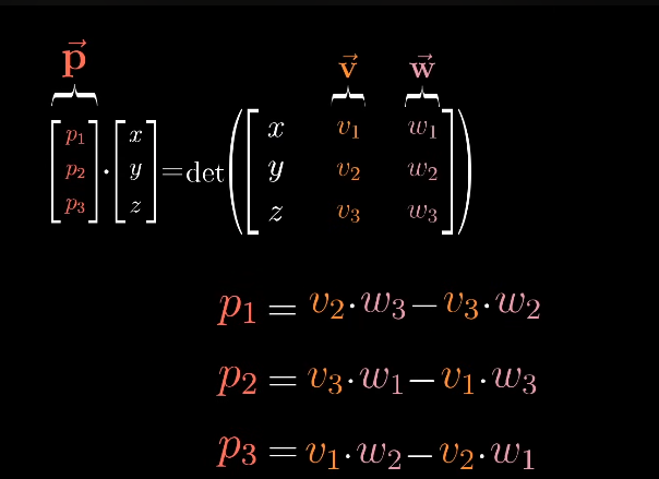
and compare coefficients, you get the actual cross product.

cramer’s rule

the good case

Say we have 2 equations and 2 unknowns:

$A\vec{x}=\vec{b}$.

$A$ is a $2\times 2$ transform.

Geometrically it is: what transform do I apply on $\vec{x}$ to make it the same as $\vec{b}$?

Now you can take an inverse and so on.

But there is a different argument too.

Initially I have $\vec{x}=\left[\begin{array}{c}x\\ y\end{array}\right]$.

Say I want to find the x-coordinate.

Area of $\vec{x}$ and $\hat{j}$:

$\det (\vec{x},\hat{j})=x$.

Area after transform: $\hat{j}\mapsto A\hat{j}$, and $\vec{x}\mapsto \vec{b}$, so area is now $\det (\vec{b},A\hat{j})$.

But this area must have been scaled by $\det (A)$:

$x\det (A)=\det (\vec{b},A\hat{j})$.

So:

$x=\frac{\det (\vec{b},A\hat{j})}{\det (A)}$.

change of basis

When we apply a transform $A$ on $\vec{x}$ that doubles $\hat{i}$, the resulting vector is $2x$ in the x direction because our basis is still the same.

Basis is how we define our vector relative to.

Had I scaled my basis, ${\hat{i}}^{\prime }=2\hat{i}$, then my vector would be the same.

A vector is just scalars saying move $a$ units in basis 1 direction, then $b$ units in basis 2 direction, and so on:

$a{\vec{b}}_1+b{\vec{b}}_2+\cdots$.

Denote $B$ as the change-of-basis matrix. For a transform $A$, this is a bit reverse.

If ${\vec{x}}_{\text{theirs}}=B{\vec{x}}_{\text{mine}}$ and $T$ is defined in their basis, then:

${\vec{x}}_{\text{mine}}^{\prime }=B^{-1}TB{\vec{x}}_{\text{mine}}$.

So the effective transform in mine is:

$B^{-1}TB$.

eigenvectors and eigenvalues

Under any transform $A$, there may exist certain vectors that only change in scale:

$A\vec{v}=\lambda \vec{v}$.

Such vectors are called eigenvectors, and the scale change is the eigenvalue. So eigenvectors and eigenvalues are closely paired.

Move everything to one side:

$A\vec{v}-\lambda I\vec{v}=0$.

So:

$(A-\lambda I)\vec{v}=0$.

For this to have a nonzero solution, the determinant must be 0:

$\det (A-\lambda I)=0$.

Once you get $\lambda$, substitute and solve $(A-\lambda I)\vec{v}=0$.

Exclude $\vec{v}=\vec{0}$.

The span of the eigenvectors is the eigenspan. If that eigenspan also spans the current space, you can choose an eigenbasis from it.

Under eigenbasis, each component of the basis is transformed separately by simple scaling by eigenvalue.

So if it exists, the $A$ transform would just be a diagonal matrix with eigenvalues on the diagonal.

This is called diagonalisation.

Say I want to calculate $A^{100}$ now. Under eigenbasis, that is cheap:

$D^{100}=\left[\begin{array}{cc}{\lambda }_1^{100}& 0\\ 0& {\lambda }_2^{100}\end{array}\right]$.

You can combine that with change of basis:

$B^{-1}{D}^{100}B$.

abstracting out the geometry

You can think of “axioms” as an interface. I define some constraints, here linearity:

$L(x+y)=L(x)+L(y)$ and $L(kx)=kL(x)$.

If whatever you have follows that, you can do all sorts of things on that.

For example, polynomials and derivatives can fit into the same linearity framework.

It will not be possible to visualise polynomials just as easily as lines and planes, but everything still holds. This is abstracting out the geometry.