readalong notes on the mml book

Chapter 2 - Basics

I think the initial chapters are REAAALY jargon heavy for no reason

linear mappings

these are the same as the scalar mappings which basically ASK something about the vector but in this case they map to a diff vector space which is fine ig, more generalised

for example R^2 ⇒ Complex numbers

Problem: say a linear map exists from vec space V → W, when would this map be bijective ( this is called isopmorphic linear map )

T : V → W bijective so inverse map to be existing ⇒ square ⇒ dim(V) = dim(W) and since inverse ⇒ full rank = rank(T) = dim(V) = dim(W)

image and kernel

kernel is the null space of a transformation T image is what’s NOT the null space ⇒ range or span under T

Fundamenta theorem of linear mappings, under transform T : V → W dim(im) + dim(null space) = dim(V)

which seems kind of obvious if you thing of a transformation as a possible collapse

affine spaces

think of an affine space as spaces with a lost origin then you would need TWO points to define a vector these spaces basically define operations in terms of two points

now say a vector space is V, set of points A, addition is allowed on these points so P + v→ from P move in v→ direction ( P becomes origin ) to get to Q which should belong to A

again redundant defns tbh

similarly u have mappings and subspaces

problem notes

• remember that both col and row ops are allowed in rank finding and det but only row when you’re reducing and augmented matrix
• ranks are defined for any matrix, just get it into echelon form and count pivots.
• pivot is non free, non pivot cols ( dims ) are free
• the full rank nullity is: rk + null = domain, rk - null = img
• automorphism ( bijective, A → A and REVERSIBLE ) and endomorphism A → within A ( structure preserving )
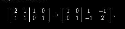
• don’t forget the augmented matrix can also be used for finding inverse.
• homomorphism → linear mapping
• for change of basis, remember that P = ( b1, b2, b3 ) where b1 is the other basis in my/std coords, then Px → converts coords in other basis to my/std. Think as x1 in b1 dir, x2 in b2 dir ( defined in my coords)… then you you apply the transform, it just gives you the final vector as transformed but in my coords.

P(bi written in std) x(in b) ⇒ x(in std)

Chapter 3 - Geometric interpretations

note: $\mapsto$ is the “maps to” operator

Norm - euclidean distance

it’s a scalar mapping, from vector space $V$ to $R$ denoted as $||x||$ or $||x|{|}_2$ ( L2 norm )

there is also $|x|$ which is the manhattan dist. aka the L1 norm $||x|{|}_1$

inner products ( abstract )

define an inner product as

$\Omega :V\times V\to \mathbb{R}$ such that it is a bilinear mapping

bilinear means that both the arguments ARE linear independently. also these can be represented as matrix ops that yield a 1x1 matrix

Anxioms ( all inner products must follow )

• symmetric ( dist a to b is same as dist b to a)
• linearity ( dist of ka same as k times dist of a )
• positive definite ( an inner product with itself > 0 for any non zero input ) no ⇐0 outputs allowed unless vec is 0

note that positive definite is only defined for self ⇒ (x,x) as args

dot product ( projections )

a dot product is ONE bilinear mapping

$x\cdot y=x^{\top }y$

these allow to define projections. dot product magnitude = project $x$ on $y$ and multiple the project length and the other vector’s length.

Why such an ugly defn of multiplying the other vec? Well it allows for really elegant computational definition so I guess it’s fine.

symmetric matrices

$A=A^{\top }$

symmetric matrices can be proved to have REAL eigenvalues ( you basically prove lambda = labda condujgate)

quadratic form of a matrix

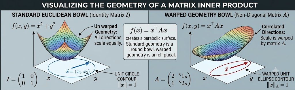
Now defne an inner product, calling it “quadratic form of matrix” as

$⟨x,y⟩=x^{\top }Ay$

Note that you can compute above for ANY matrix, but for it to be an inner product, only matrices are allowed and that this those that satisy the positive definite rule.

This is also called as the “warped geometry bowl” based on how it looks in the 3d space of (x,y,f(x,y))

norm as inner product

$\Vert x\Vert :=\sqrt{⟨x,x⟩}$

but not every norm can be an inner product, example L1 norm.

general form of Cauchy-Schwarz inequality

$|⟨x,y⟩|\le \Vert x\Vert \Vert y\Vert$

where RHS is L@ norms.

metric

an inner product used to define distance. the same rules as inner product apply except you also need triangle inequality.

angles

from Cauchy-Schwarz, if you remove the abs on left, you get

$-1\le \frac{⟨x,y⟩}{\Vert x\Vert \Vert y\Vert }\le 1$

Now think of cosine func, if you restrict input from to pi then it uniquely maps the range [-1,1].

so this above can be $cos(\theta )$ where $\theta$ is the angle.

Now this’ll be the angle in 2d plane that I’m familiar with if the inner product happens to be a dot product, otherwise it’s SOME angle.

orthonormal

which brings us to perperdicularity and how it relates to basis ( a sheared basis may not retain same perpendicular vectors )

orthogonal ⇒ inner product is 0 normal ⇒ L2 norm is 1

orthonormal ⇒ both above

orthogonal matrix

• (n,n) matrix
• $A{A}^{\top }=I=A^{\top }A$

aka transpose is inverse.

to be orthogonal, you need column vectors to be ortho (pairwise) and normal.

any transformation UNDER an orthogonal matrix, preserves ANGLE and DISTANCE.

using this as a basis is an orthonormal basis.

orthogonal complement

for a space V ( as the vec space ) and U as a subspace in it

ortho complement is set of { perpendiculars to each vector in U, that exist in V }

inner product of funcs

think of a high dimentional dot product

$⟨u,v⟩={\sum }_{i=1}^n{u}_i{v}_i=u_1{v}_1+u_2{v}_2+\cdots +u_n{v}_n$

as the dimensionas move to infinity

$\text{cont. inner product}={\int }_a^b\underset{\text{Height 1}}{\underbrace{u(x)}}\times \underset{\text{Height 2}}{\underbrace{v(x)}}\times \underset{\text{Width}}{\underbrace{dx}}$

projections

$\underset{\text{Original Vector}}{\underbrace{y}}=\underset{\text{Horizontal Projection}}{\underbrace{{\text{proj}}_x(y)}}+\underset{\text{Remaining Vertical Line}}{\underbrace{\left(y-{\text{proj}}_x(y)\right)}}$

the first part is the dot product (lenth adjusted), which defines the ACTAUL projection, second is the orthogonal projection. Together they complete the triangle.

technically, for the same inner product defn of orthogonality, you’ll use the same inner product for projection. just replace dot with whatever other innner product.

${\text{proj}}_b(x)=\left(\frac{x\cdot b}{\Vert b{\Vert }_2^2}\right)b=\left(\frac{b^{\top }x}{b^{\top }b}\right)b$

the term in brackets in last is the projection matrix of b for this projection. this above covers projections in general for lines ( 1d subspace ).

what about more dims? projecting onto a plane?

first define this for the final projection

Here is the cleaned-up version of your notes with the typos fixed and the math properly formatted in LaTeX. I kept your original logic and flow exactly the same, just polished it up so it is ready for your notes!

• $\mathbf{B}$ represents the basis in subspace $U$. Any vector in $U$ can be represented as $\mathbf{B}\mathbf{\lambda }$, where $\mathbf{\lambda }$ is a column vector of coordinates.
• This vector can be represented in the original larger space (the superspace), since the subspace belongs to it.
• To get the projection point, we know it lies within subspace $U$, so we can say it is $\mathbf{B}\mathbf{\lambda }$.
• For the final vector to have the minimal distance along ANY direction included in the basis of $U$, it must have no component along any of $\mathbf{B}$‘s columns. It must be orthogonal to each basis vector (covering the basis is enough, as every direction in the subspace is covered by it).
• But what must be orthogonal? The vector from this projection to $\mathbf{x}$ (the input we are projecting). This is $(\mathbf{x}-\mathbf{B}\mathbf{\lambda })$. In linear regression contexts, this is defined as the residual, $\mathbf{e}$.
• If we take ${\mathbf{b}}_i$ as the $i$-th basis vector, the orthogonality condition is:

${\mathbf{b}}_i^{\top }(\mathbf{x}-\mathbf{B}\mathbf{\lambda })=0$

• Stacking each of these as columns gives us the matrix form:

${\mathbf{B}}^{\top }(\mathbf{x}-\mathbf{B}\mathbf{\lambda })=0$

${\mathbf{B}}^{\top }\mathbf{B}\mathbf{\lambda }={\mathbf{B}}^{\top }\mathbf{x}$

$\mathbf{\lambda }=({\mathbf{B}}^{\top }\mathbf{B}{)}^{-1}{\mathbf{B}}^{\top }\mathbf{x}$

The coeef of $x$ in last is called the “pseudo-inverse” of B. Since $B^{\top }B$ is square, symmetric and invertible ALWAYS.

The symmetry you can kind of think as the symmetry of a projection itself ( a on b verses b on a )

GM orthogonalisation

any basis U can be converted to an orthonormal basis B with the same span. I’ll assume B always exists, and it does ( intuitively too you can think of an n dimensional space as n directions somewhere in the space and then you just define B as one unit in each of those )

GM is then a recursive ( peeling subspace dimensions as it’s often written ) algo to find this B using projections.

u_1 := choose ANY vector in B, or just b_1 for simplicity for u_k:

• define $U_{k-1}:=\text{span}({\mathbf{u}}_1,\dots ,{\mathbf{u}}_{k-1})$
• project $b_k$ orthogonal to this subspace ${\mathbf{u}}_k:={\mathbf{b}}_k-{\text{proj}}_{U_{k-1}}({\mathbf{b}}_k)$

Now this isn’t as obvious unless you are over-simplying some things. For example, we have glossed over why projections still form a span. Why would a projection not be zero? I can address that a bit by arguments? At each step we have an EXCLUDED basis, so for the span, we exclude some subspace ( what remains is what is orthogonal to that subspace ) and find vectors that exist there, since original was a span of the space, there MUST exist some component in that direction. What if this particular $b_i$ has no component in that direction? Note that as we peel dimentions, we are increasing the excluded space, for the 2nd step, the valid space is ALL - one dimension ( that of $b_1$ ), so IF it is a span ( aka linearly independent ), this is same as asking “okay, what do you have in ANY OTHER DIRECTION except $b_1$, which for a span should exist.

projections and affine spaces

this I’m skipping for now. reminder that affine spaces are spaces with a LOST or rather unspecified origin ( so you can only talk relatively OR need to define an origin as reference point )

rotations

Note that rotations is FUNDAMENTALLY a planar operation, for you always have an axis of rotation, and a plane of rotation perpendicular to it.

Hence at any level you can apply the complex number interpretation.

$z_{rotated}=z\cdot e^{i\theta }=(x+iy)(\cos \theta +i\sin \theta )$

$\mathbf{R}(\theta )=\left[\begin{array}{cc}\cos \theta & -\sin \theta \\ \sin \theta & \cos \theta \end{array}\right]$

pre-requisites on complex numbers to lin algebra

The equivalent basis vectors for $1$ and $i$ from the complex plane would be $\left[\begin{array}{c}1\\ 0\end{array}\right]$ and $\left[\begin{array}{c}0\\ 1\end{array}\right]$.

So $a+ib$ is just $a\left[\begin{array}{c}1\\ 0\end{array}\right]+b\left[\begin{array}{c}0\\ 1\end{array}\right]$.

Now if you take an initial $(x,y)$ aka $x+iy$, then multiply by $e^{i\theta }$, gives you: real $\Rightarrow x\cos \theta -y\sin \theta$ img $\Rightarrow y\cos \theta +x\sin \theta$

To get what the NEW basis vectors become, put in the old basis $\left[\begin{array}{c}1\\ 0\end{array}\right]$ then $\left[\begin{array}{c}0\\ 1\end{array}\right]$.

So $\left[\begin{array}{c}1\\ 0\end{array}\right]$ becomes $x\cos \theta +ix\sin \theta$, which is $\left[\begin{array}{c}\cos \theta \\ \sin \theta \end{array}\right]$.

Similarly for the other, $\left[\begin{array}{c}0\\ 1\end{array}\right]$ becomes $\left[\begin{array}{c}-\sin \theta \\ \cos \theta \end{array}\right]$.

rotations in higher dimentions

Now since there’s an axis of rotation, I can ALWAYS decompose rotation along the basis axes (or any other axis represented in that basis) and COMBINE them by an equivalent transform.

For example, define ${\mathbf{R}}_y$ to be using $y$ as the axis $\Rightarrow$ anything in the $y$ direction is UNCHANGED and has the equivalent of what an identity matrix would have, for the rest you have the same absolute terms as the ${\mathbb{R}}^2$ case, except with $(-1{)}^{i+j}$ sign multiplications to account for clockwise/counterclockwise.

${\mathbf{R}}_y(\theta )=\left[\begin{array}{ccc}\cos \theta & 0& \sin \theta \\ 0& 1& 0\\ -\sin \theta & 0& \cos \theta \end{array}\right]$

Similarly in $n$ dimensions.

Now 2 dimensions made the axis and the plane CLEAN as the axis is cleanly defined as what’s perpendicular to the plane (and passing through the origin).

In the $n$-th dimension, this is not unambiguous as perpendiculars exist in many dimensions so you define the 2D plane instead.

$n$-th basis $\Rightarrow$

$${\mathbf{R}}_{ij}(\theta ):=\left[\begin{array}{ccccc}{I}_{i-1}& 0& \dots & \dots & 0\\ 0& \cos \theta & 0& -\sin \theta & 0\\ 0& 0& I_{j-i-1}& 0& 0\\ 0& \sin \theta & 0& \cos \theta & 0\\ 0& \dots & \dots & 0& I_{n-j}\end{array}\right]\in {\mathbb{R}}^{n\times n}$$

$I_k$ is just an identity matrix block of $k$ size. Just notation to skip the … in essence, they are what would be in an identity matrix of $n_{th}$ dimension.

This covers rotation.

note: one property that’s a bit non-obvious is that rotation is ONLY commutative in $R_2$ and not in higher dimensions.

Think of a R3 rotation as composed of two R2 ones ( it has to be this way ) and then just say that matrix multiplication is not commutative.

problens

• when basis is orthogonal, you can define an orthogonal projection to a subspace U as the sum of projections on the individal basis vectors. ( this is only when it’s orthogonal basis as otherwise you would be double counting contributions on cases where different basis vectors cover components in the same direction )
• inner product with self can very much be > 0, even dot product is; this I was confusing with the distance meric, define as root of self dot of x-y
• projection as an operator ( not as a vector result ) is defined as any transformation that is idempotent so ${\pi }^2=\pi$
• a better intuition of rank nullity ⇒ T takes it from V to W ⇒ output ( image )= input ( V ) - lost ( kernel )
• $1_n$ is notation for an n dimensional all 1 vector.
• a better way to remember CS ⇒ $dotproduc{t}^2<=(sumofsquares)(sumofsquares)$

Chapter 4 - Matrix Decompositions

Determinants

same as what I’ve covered already mostly.

det computation via laplacian expansion is slow, what’s usually done is Gaussian elim or LU decomp.

In gaussian elim, in the row echelon matrix, the product of diagonal elems give you the det ( of the echelon matrix) Then you reverse back the linear transforms applied on rows to get the original one back

Trace

sum of diagonal entries. this is a special and UNIQUE function with these properties

• linearity
• cyclic rot invariant

you can use this commutativity to simplify $tr(x{y}^T)$ which would be $n\times n$ to $tr(y^{T}x)$ which is just the dot product.

applying the 2nd property, you can get that trace is basis invariant.

characteristic polynomial

$p_A(\lambda ):=\det (A-\lambda I)$

I don’t think there’s any signficance to this along, other than a polynomial with eigenvalues as root. But I could be ignorant here.

The book went in the other direction, defining this first and the eigenvalues as it’s root. I think that’s not the right way to introduct this topic.

Eigenvalues and eigenvectors

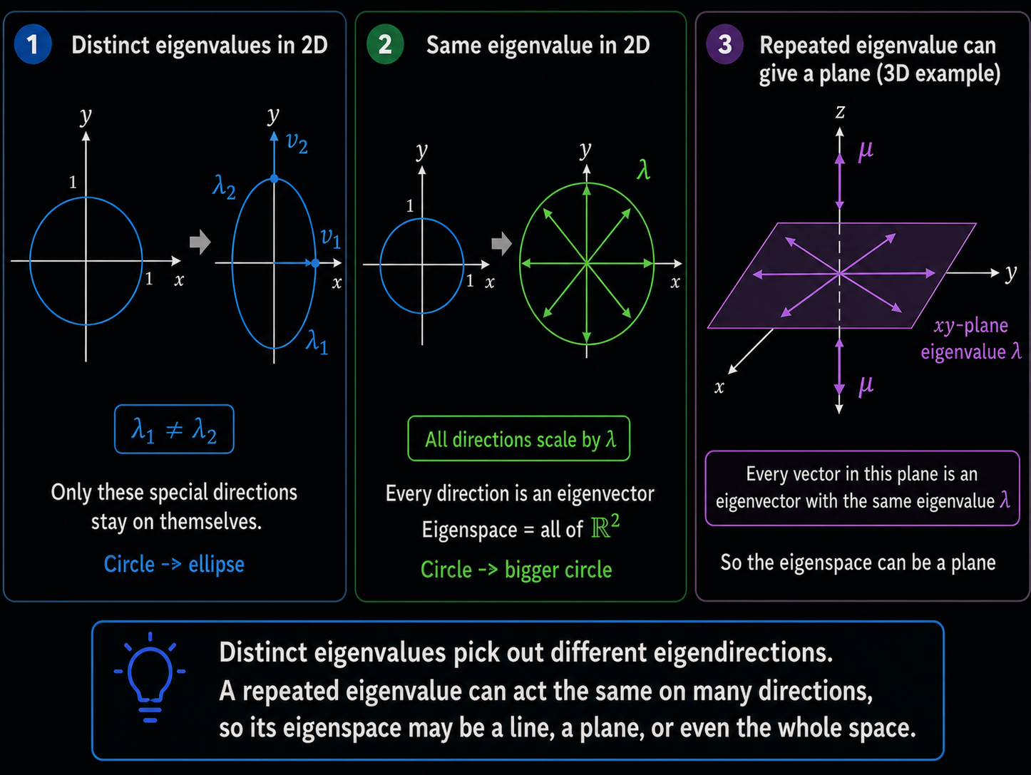
For a given eigenvalue, you atleast have infinite eigenvectors ( as collinear ones count too ). Can define that line as the eigenspace.

If multiple eigenvectors share the same value, they will all belong to the same eigenspace and increase it’s dimensions. For example, if it becomes a plane, it means the transformation scale the same amount in every direction on that plane. Consider a cicle and ellipsis as scaling cases. This number of LI eigenvectors is called the geometric multiplicity of that eigenvalue.

Set of all eigenvalues of $A$ is called the spectrum of $A$.

eigenvalues are transpose invariant ( not vectors ). This comes form det being transpose invariant.